Simultaneous feature preprocessing, feature selection, model selection, and hyperparameter tuning in scikit-learn with Pipeline and GridSearchCV

Introduction

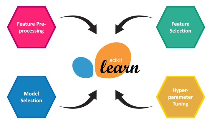
Some of the key steps in a machine learning workflow are:

• feature preprocessing (encoding categorical features, scaling numeric features, transforming text data, etc.);
• feature selection (choosing which features to include in the model);
• model selection (choosing which machine learning estimator to use); and,
• hyperparameter tuning (determining the optimum hyperparameter values to use for each estimator).

It can be difficult to perform these tasks in an accurate, efficient and reproducible manner. In particular, it is important to ensure that, during cross-validation, feature preprocessing and feature selection are based only on the training portion of data, preventing leakage from the validation set which could bias our results. In this short, practical post I’ll demonstrate how to use scikit-learn to simultaneously perform the above steps. While the example given is somewhat contrived, the syntax and workflow are what is important here and can be applied to any machine learning workflow.

Step 1: Import dependencies

from sklearn.pipeline import Pipeline
from sklearn.datasets import make_classification
from sklearn.preprocessing import StandardScaler
from sklearn.model_selection import GridSearchCV
from sklearn.neighbors import KNeighborsClassifier
from sklearn.linear_model import LogisticRegression
from sklearn.ensemble import RandomForestClassifier
from sklearn.feature_selection import SelectKBest, mutual_info_classif
pd.options.plotting.backend = "plotly"

Step 2: Import data

We will create a synthetic binary classification dataset for this demonstration using the scikit-learn function make_classification.

X, y = make_classification(n_samples=1000,
                           n_features=30,
                           n_informative=5,
                           n_redundant=5,
                           n_classes=2,
                           random_state=123)

The plot below shows 100 random points sampled from this synthetic dataset, with only the first two features used for plotting purposes.

Step 3: Create pipeline framework

Using our synthetic dataset, we are going to set up a pipeline object that will:

• Standardize the data using StandardScaler;
• Select the k best features from the data using SelectKBest and the mutual information metric (where k is a hyperparameter that we will tune during the fitting process); and,
• Use an estimator to model the data, here we will be trying a LogisticRegression, RandomForestClassifier, and KNeighborsClassifier.

The syntax for creating this pipeline is shown below. To instantiate the Pipeline object I’ve used a k value in SelectKBest of 5 and I’ve input LogisticRegression as the estimator, but these are simply placeholders for now and they will be varied during the fitting stage.

pipe = Pipeline([('scaler', StandardScaler()),
                 ('selector', SelectKBest(mutual_info_classif, k=5)),
                 ('classifier', LogisticRegression())])

Step 4: Create search space

The next step is to define the space of hyperparameters and estimators we want to search through. We do this in the form of a dictionary and we use double underscore notation (__) to refer to the hyperparameters of different steps in our pipeline. We will be trying out different values of k for the feature selector SelectKBest, as well as different hyperparameter values for each of our three estimators as shown below.

search_space = [{'selector__k': [5, 10, 20, 30]},
                {'classifier': [LogisticRegression(solver='lbfgs')],
                 'classifier__C': [0.01, 0.1, 1.0]},
                {'classifier': [RandomForestClassifier(n_estimators=100)],
                 'classifier__max_depth': [5, 10, None]},
                {'classifier': [KNeighborsClassifier()],
                 'classifier__n_neighbors': [3, 7, 11],
                 'classifier__weights': ['uniform', 'distance']}]

Step 5: Run the GridSearch

This is where the magic happens. We will now pass our pipeline into GridSearchCV to test our search space (of feature preprocessing, feature selection, model selection, and hyperparameter tuning combinations) using 10-fold cross-validation

clf = GridSearchCV(pipe, search_space, cv=10, verbose=0)
clf = clf.fit(X, y)

Step 6: Get the results

We can access the best result of our search using the best_estimator_ attribute. For this particular case, the KNeighborsClassifier did the best, using n_neighbors=3 and weights='distance', along with the k=5 best features chosen by SelectKBest. This combination had a 10-fold cross-validation accuracy of 0.958.

clf.best_estimator_

Pipeline(memory=None,
         steps=[('scaler',
                 StandardScaler(copy=True, with_mean=True, with_std=True)),
                ('selector',
                 SelectKBest(k=5,
                             score_func=<function mutual_info_classif at 0x15610c3b0>)),
                ('classifier',
                 KNeighborsClassifier(algorithm='auto', leaf_size=30,
                                      metric='minkowski', metric_params=None,
                                      n_jobs=None, n_neighbors=3, p=2,
                                      weights='distance'))],
         verbose=False)

clf.best_score_

0.958